In-class_Ex06

Published

February 13, 2023

Modified

March 27, 2023

1 Overview

1.1 Install and load packages

pacman::p_load(sf, sfdep, tmap, tidyverse)

2 DATA

2.1 Import Geospatial Data

hunan <- st_read(dsn = "data/geospatial", 
                 layer = "Hunan")

Reading layer `Hunan' from data source 
  `C:\kt-x\is415-GAA\In-class_Ex\In-class_Ex06\data\geospatial' 
  using driver `ESRI Shapefile'
Simple feature collection with 88 features and 7 fields
Geometry type: POLYGON
Dimension:     XY
Bounding box:  xmin: 108.7831 ymin: 24.6342 xmax: 114.2544 ymax: 30.12812
Geodetic CRS:  WGS 84

2.2 Import Aspatial Data

hunan2012 <- read_csv("data/aspatial/Hunan_2012.csv")
hunan2012

# A tibble: 88 × 29
   County    City     avg_w…¹ depos…²    FAI Gov_Rev Gov_Exp    GDP GDPPC    GIO
   <chr>     <chr>      <dbl>   <dbl>  <dbl>   <dbl>   <dbl>  <dbl> <dbl>  <dbl>
 1 Anhua     Yiyang     30544  10967   6832.    457.   2703  13225  14567  9277.
 2 Anren     Chenzhou   28058   4599.  6386.    221.   1455.  4941. 12761  4189.
 3 Anxiang   Changde    31935   5517.  3541     244.   1780. 12482  23667  5109.
 4 Baojing   Hunan W…   30843   2250   1005.    193.   1379.  4088. 14563  3624.
 5 Chaling   Zhuzhou    31251   8241.  6508.    620.   1947  11585  20078  9158.
 6 Changning Hengyang   28518  10860   7920     770.   2632. 19886  24418 37392 
 7 Changsha  Changsha   54540  24332  33624    5350    7886. 88009  88656 51361 
 8 Chengbu   Shaoyang   28597   2581.  1922.    161.   1192.  2570. 10132  1681.
 9 Chenxi    Huaihua    33580   4990   5818.    460.   1724.  7755. 17026  6644.
10 Cili      Zhangji…   33099   8117.  4498.    500.   2306. 11378  18714  5843.
# … with 78 more rows, 19 more variables: Loan <dbl>, NIPCR <dbl>, Bed <dbl>,
#   Emp <dbl>, EmpR <dbl>, EmpRT <dbl>, Pri_Stu <dbl>, Sec_Stu <dbl>,
#   Household <dbl>, Household_R <dbl>, NOIP <dbl>, Pop_R <dbl>, RSCG <dbl>,
#   Pop_T <dbl>, Agri <dbl>, Service <dbl>, Disp_Inc <dbl>, RORP <dbl>,
#   ROREmp <dbl>, and abbreviated variable names ¹avg_wage, ²deposite

2.3 Combine both df using left-join

Always do left-join cause its best to put the sf df the left side then right side is the tibble

hunan_GDPPC <- left_join(hunan, hunan2012) |>
  select(1:4, 7, 15)

NOTE: during joining,must have a common field (unique identifier) then another thing to take note is to make sure both columns have same number of attributes(?)

2.4 Plotting Chrorpleth map

tmap_mode("plot")
tm_shape(hunan_GDPPC)+
  tm_fill("GDPPC", 
          style = "quantile", 
          palette = "Blues",
          title = "GDPPC") +
  tm_layout(main.title = "Distribution of GDP per capita by district",
            main.title.position = "center",
            main.title.size = 1.0,
            legend.height = 0.45, 
            legend.width = 0.35,
            frame = TRUE) +
  tm_borders(alpha = 0.5) +
  tm_compass(type="8star", size = 2) +
  tm_scale_bar() +
  tm_grid(alpha =0.2)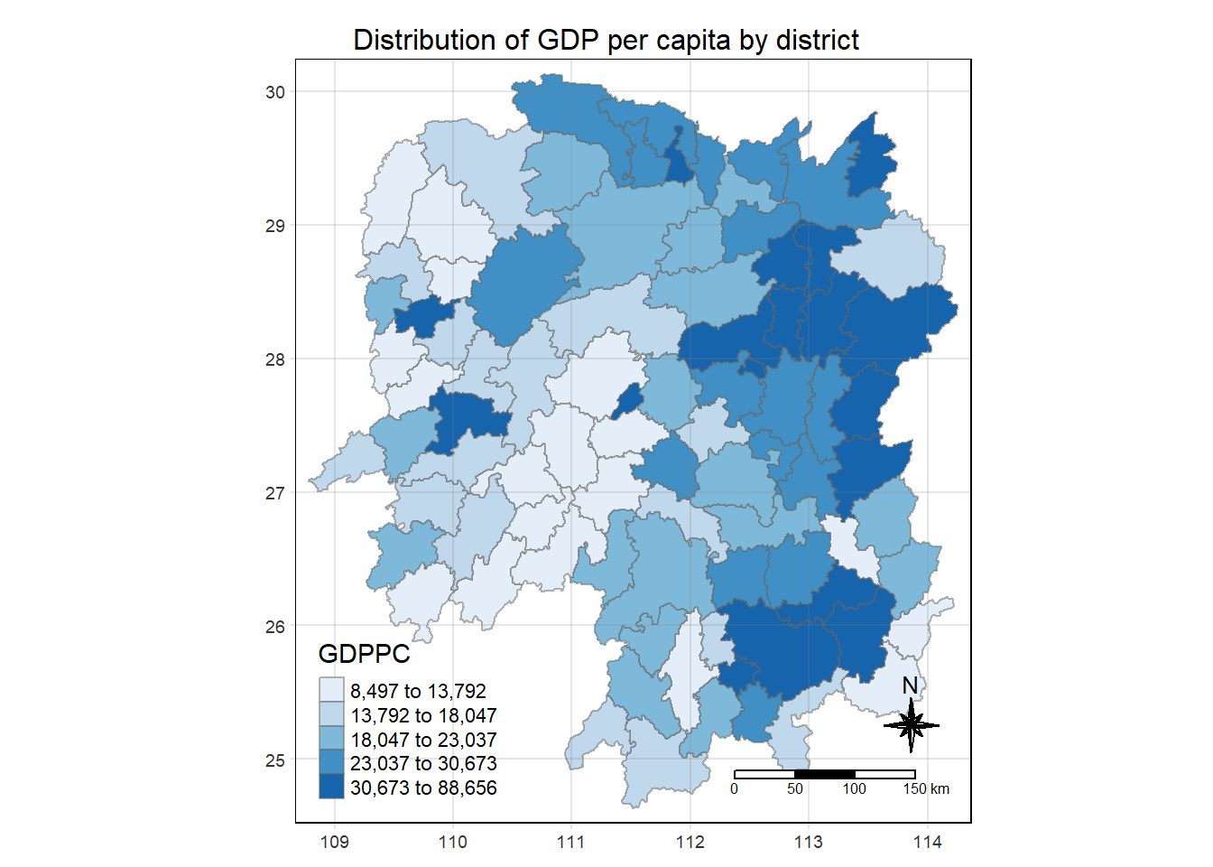

3 Identify neighbours

3.1 Contibuity neighbours method

.before = 1 is to put the newly created column at the first column onwards.

cn_queen <- hunan_GDPPC |>
  mutate(nb = st_contiguity(geometry), .before = 1)

3.2 Neighbour list by Rook’s method

queen = false is to know that the default queen is false then its rook.

cn_rook <- hunan_GDPPC |>
  mutate(nb = st_contiguity(geometry), queen = FALSE, .before = 1)

wm_q = hunan_GDPPC |>
  mutate(nb = st_contiguity(geometry), 
         wt = st_weights(nb), 
         .before = 1)

3.3 Contiguity rook method

wm_r = hunan_GDPPC |>
  mutate(nb = st_contiguity(geometry), 
         queen = FALSE,
         wt = st_weights(nb), 
         .before = 1)